If you need help navigating Photon Engineering's FRED or understanding its features, check out our helpful videos and articles. Whether you're just starting or looking to dive deeper into advanced functionalities, our resources offer clear instructions to guide you through every step. Explore the articles to enhance your knowledge and make the most of FRED's capabilities.
Photon Engineering adheres strictly to the OpenGL standard, but sometimes graphics card drivers can cause issues. To improve the performance of your 3D visualization view, try the following:
Change the pixel format preference:
Navigate to Tools > Preference from the menu.
Click on the Visualization tab.
Set the pixel format to “Fast.”
Note: This change will not take effect until you open a new FRED document.
By following these steps, you may enhance the responsiveness of your 3D visualization view.
To resolve freezing or crashing problems in your 3D visualization view, consider the following solutions:
Adjust Pixel Format:
Go to Tools > Preferences from the menu.
Click on the Visualization tab.
Set the pixel format to “Safe” to enforce a software rendering mode.
Note: Changes to FRED preferences take effect only when a new FRED document is opened.
2. Use the GLView.exe Utility:
Utilize the GLView.exe utility included with your FRED installation to find an acceptable OpenGL hardware rendering mode for your graphics card.
Generally, choose a pixel mode where the “letter cube” in the GLView.exe utility rotates smoothly without flickering (this may not be the fastest rotation).
3. Update Video Drivers:
Download and install the latest video drivers from your graphics card manufacturer’s website.
By following these steps, you should be able to improve the stability of your 3D visualization view.
By default, FRED autosaves one “level of undo” in the Undo directory. You can undo one action by selecting Edit > Undo from the menu. This action is stored in a .fru file or a .frs script in the Undo directory.
To increase the number of autosaved FRED documents, select Tools > Preferences from the menu, then click on the Miscellaneous 2 tab. Use the up or down arrows to change the “number of levels of undo.” The autosaved .fru files are named “FREDUndoXXXXXXX_Y.fru,” where X represents the timestamp of the autosave, and Y indicates the undo level. However, FRED only autosaves the most recent script file as MostRecentScript.frs.
To recover a .fru file, locate the Undo directory and change the file’s extension from .fru to .frd. You can then open or move this file as you normally would.
To recover the most recent script file, find it in the Undo directory and open it as you would any script file. You can then save this file as you normally would.
Note: The default Undo directory is C:\Documents and Settings<username>\Local Settings\Temp\Fred Undo. You can change this by selecting Tools > Preferences > File Locations from the menu, scrolling through the file list, and editing the entry for “Undo directory.”
Another Note: To have FRED automatically search the Undo directory and recover the most recent .fru document, ensure “Allow abort recovery” is selected as a preference. To do this, select Tools > Preferences, click on the Miscellaneous tab, and check the “Allow abort recovery” checkbox.
Hyper-threading technology creates virtual CPU cores that do not function the same way as physical CPU cores. As a result, the anticipated linear speed scaling may not occur. Performance scaling can also depend on the specific construction of your FRED model. For instance, the types and organization of surfaces within the model influence how effectively the raytrace can scale with the number of threads. Additionally, keep in mind that the Trace and Render option for a raytrace operates as a single-threaded calculation, meaning it does not utilize the additional cores of your computer.
FRED’s user interface is highly flexible and customizable, allowing toolbars and windows to be floated or docked anywhere on the screen. If something has been moved off the screen or is no longer visible, you can restore it.
For a Lost Toolbar:
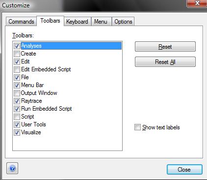
Go to View > Customize > Toolbars from the menu.
Click on the Reset button to restore the toolbar.
For a Lost Window (e.g., the Output Window):
If resetting the toolbar doesn't resolve your issue, follow these steps to restore a lost window:
Open a Command Prompt in Windows.
Change to the Bin directory of your FRED installation. For example, type:
cd "C:\Program Files\Photon Engineering\FRED 14.40.0\Bin"
Run the FRED executable with the command line option:
Fred.exe /NoLoadWindowStates
This command will reset the window settings to their default state, allowing you to regain access to any lost windows.
To model a partially coherent source in FRED, simulate an extended source as a collection of point sources. These sources should be positioned at different locations (for finite conjugates) or directed in various ways (for infinite conjugates). While each individual source will remain coherent, they will be incoherent with respect to one another.
Here's how to set this up in FRED:
Use Different Wavelengths: Assign different wavelengths to each point source to simulate partial coherence.
Example File: A practical example of implementing a partially coherent source can be found in the FRED Sample Files folder at the following path: <installation dir>\Resources\Samples\Tutorials & Examples\examplePartialCoherenceDiffractometer.frd.
Modeling a solar source in FRED can be approached in different ways depending on the accuracy required for your simulation. The parameters to consider include the time of year, time of day, geographic location (longitude and latitude), and weather conditions. Here’s a simple method to create a solar source:
Create a Plane Source:
Set up a plane source with randomized ray positions and directions within an angular range that represents the subtense of the solar disk (approximately 0.5°).
Define Wavelengths:
Add wavelengths and weightings that are appropriate for a blackbody source like the sun. This can be done by creating a blackbody spectrum.
Adjust for Atmospheric Conditions:
Scale the wavelength weights according to atmospheric transmission values to account for weather or regional conditions.
Set Source Power:
Configure the power of the source in the Power tab to reflect the solar irradiance value and the size of the system aperture.
For a more automated approach, you can use the Solar Source (simple) type of Source Primitive, which implements the above method semi-automatically.
For advanced modeling, consider utilizing theories such as the Bird Model (available at NREL). This model accounts for diffuse radiance from the atmosphere, which can be treated as isotropic, and provides specific data regarding the wavelength spectrum.
FRED utilizes a third-party chart control tool from Component One, LLC, for displaying and processing visual data. This tool offers advanced settings and features that can be modified within FRED. For additional help, two documents related to the 2D and 3D chart controls are located in the directory C:\Windows\Help\, named olch2d8u.chm and olch3d8u.chm. You can also access chart help by right-clicking in the chart view, selecting Advanced from the menu, and clicking the Help button.
Customization Procedure
To customize your chart views, follow these steps:
With a chart open in FRED, adjust the settings using the FRED menu options or the advanced controls available by right-clicking in the chart view. For detailed documentation on the advanced controls, refer to the help content mentioned above.
After selecting your desired settings, open the advanced chart controls by right-clicking in the chart view and choosing Advanced from the menu.
In the advanced controls dialog, select Save from the Control tab. This will create a file containing the specifications for your current chart settings.
In FRED, open the Preferences dialog by navigating to Menu > Tools > Preferences, and select the File Locations tab.
In the File List area, choose the chart type you wish to customize, then use the File Location browser to select the saved file from step 3.
Press OK to accept the settings. The next plot window will reflect your customizations.
By following these steps, you can effectively customize your charts in FRED to better suit your visual data needs.
This error message usually indicates that security software is likely interfering with FRED’s read/write operations. We recommend consulting your IT department to check for any recent updates or changes to your security software that might be causing this issue.
This issue may occur when the minimum free hard disk space is less than the amount needed for the Ray Buffer pagefile. For more details and solutions, please refer to the article “FRED Preference Optimization.”
This error typically occurs when the minimum free hard disk space is less than what is required for the Ray Buffer pagefile. For more information and troubleshooting steps, please refer to FRED’s Online Help topic “FRED Preference Optimization.”
The parametric construction of NURB surfaces differs fundamentally from other native FRED surfaces, making it challenging to position or attach analysis surfaces to NURBs. While native FRED surfaces have a definite, known origin, imported CAD models may have NURB surfaces with arbitrary shapes, sizes, and positions. This raises the question of which point on the NURB surface becomes the origin after import. For a detailed guide on attaching analysis planes to NURB surfaces, please refer to the article, “CAD Surface Position and Orientation.”
If you are confident that the surface information is correct, the issue is most likely related to visualization settings. Try increasing the tessellation (i.e., decreasing the tessellation scale size) for the selected entities to improve the surface's appearance. For further details on adjusting visualization attributes, please refer to FRED’s Online Help topic, “Visualization Attributes.”
This error occurs when running a script in FRED version 9.50 or earlier after saving a document as a *.frs file. To resolve this issue, remove the lines “Sub Main” and “End Sub” from the script file before running it. This adjustment should prevent the error and allow the script to run properly.
To manipulate the position and orientation of an object using FRED’s scripting language, use the T_OPERATION structure along with the linear transformation commands. You can find a comprehensive list of these commands in FRED’s Online Help topic, “FRED Commands by Usage.” Additionally, in the article, “Rotating Prisms by Scripting,” provides an example of scripting object position and orientation. For more detailed discussions and further examples, refer to FRED’s Online Help topic titled “Position / Orientation.”
In FRED v9.50 and later, script commands are divided into application-level and document-level commands. Application-level commands (e.g., math commands, file commands) can be run without an open FRED document. However, document-level commands require an associated FRED document to be recognized by the script editor.
If only one document is open, FRED automatically associates the script with that document. If multiple documents are open, you need to manually associate the script with a specific document. To do this, go to Script > Associate with FRED Document in the menu, select the document, and click OK.
Yes, FRED offers multiple options for automation and scripting:
FRED has a built-in BASIC scripting language, which is highly useful for automating tasks and creating custom workflows.
FRED can also be controlled externally via COM (Component Object Model), allowing integration with programming environments such as Python, MATLAB, and VB.
This flexibility enables users to automate processes, run simulations, and interact with FRED seamlessly through their preferred tools.
When FRED is installed on a computer for the first time, the default settings are configured to prioritize program stability rather than fully utilizing the machine's resources. These initial settings are intentionally conservative to ensure reliable operation. This article outlines the key preference adjustments you should make after installing FRED to enhance the graphical user interface (GUI) and improve the performance of raytracing and analyses.
It is advisable to launch FRED, apply the recommended changes detailed in this guide, and then close the application. Doing so ensures that the modifications are properly saved to the system registry.
GUI Preferences
Ray Buffer Preferences
Graphical User Interface Settings
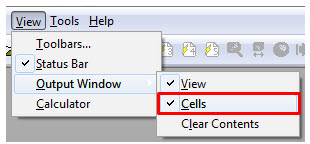
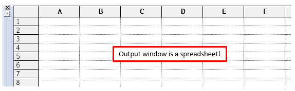
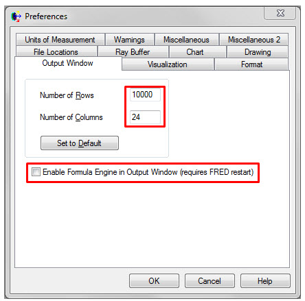
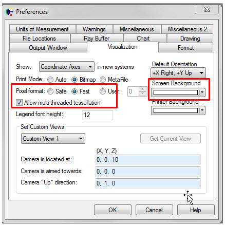
Navigate to the View menu and toggle the Cells option of the Output Window sub-menu. This option allows to view the Output Window as a spreadsheet (which it is) rather than as an empty text window. Next, open up the Preferences dialog by navigating to Tools > Preferences. The Output Window tab allows you to control how many rows and columns are available at any given time. To maintain a comprehensive history in the Output Window for easier navigation and review of FRED outputs, it is recommended to set the preferences to 10,000 rows and 24 columns. Additionally, consider disabling the formula engine if it is not required for your workflow, as this can help avoid potential issues and improve stability. Next, move to the Visualization tab and make the following changes:
Pixel Format = Fast
Allow multi-threaded tessellation = Checked
The screen background color can be customized based on your preference, with common choices being black or white. This is the section where you can adjust this setting to suit your visual preferences.
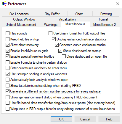
The Pixel Format setting controls whether the 3D view uses a “software” rendering mode or hardware acceleration using your graphics card. The Fast option tells FRED to use the graphics card acceleration. Multi-threaded tessellation is exactly what it indicates. When the 3D view needs to be redrawn, FRED will use as many CPU cores as are available. Move to the Miscellaneous tab of the Preferences dialog and duplicate the options below.
Enable IntelliMouse in Grids – this option allows mouse wheel scrolling in dialogs that use grids. This includes the Output Window!
Enable Formula Engine in certain dialogs – uncheck this for the reason mentioned above
Enter Curvatures – uncheck this, unless you are a crazy person and prefer to think in a manner that is the reciprocal of the way rational people think
Use isotropic scaling in analysis windows – opens chart windows with the view scaled proportionally to the analysis grid axes
Display enhanced raytrace statistics – toggle this and you will get additional information printed to the output window following a raytrace
Generate curve enclosure masks – make sure this is toggled so that certain surface types with complex apertures use “enclosure masks” to help with raytrace efficiency
Show dashboard on startup - will display the dashboard when you start FRED allowing you quick access to various functions, licensing information, and Help information
Ray Buffer Preferences
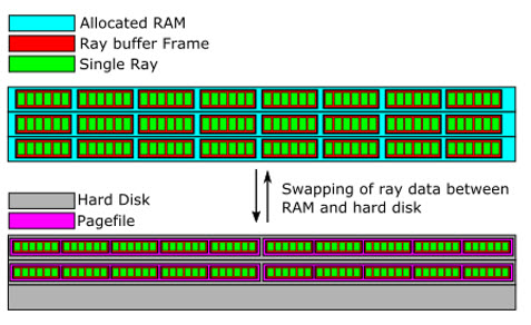
To optimize FRED's performance, it is essential to configure the settings in the Ray Buffer tab of the Preferences dialog. Before diving into specific configurations, it is helpful to understand how the ray buffer operates. Ideally, all ray data should be stored in RAM for rapid access. However, over-utilizing RAM can lead to unpredictable program behavior or system instability, even though Windows attempts to manage such situations effectively.
By default, FRED allocates a small portion of RAM for storing ray data. While this ensures stability, it limits the amount of ray data that can be stored in memory. If more rays are generated during a trace than the allocated RAM can accommodate, FRED temporarily stores the excess ray data in “pagefiles” on the hard drive. This process allows for continued operation but impacts raytracing performance, as accessing data from RAM is significantly faster than from a hard drive, although the performance gap is reducing with advancements in storage technology.
The concept can be illustrated as follows: a “frame” in FRED represents a finite-sized block of RAM allocated for storing a specific number of rays. The total number of frames and the rays per frame are user-defined settings. Their product determines the maximum number of rays that can reside in RAM at any moment, effectively dictating the RAM allocated for FRED's ray buffer.
For example, if six rays are stored per frame and 24 frames are allocated, the total capacity is 6×24=144 rays in RAM at any time. If a raytrace produces more than 144 rays, the additional data is stored in pagefiles on the hard drive and swapped back into memory as needed. While this system maintains functionality, optimizing the allocation can significantly improve performance. So what are the general rules for optimizing the ray buffer preferences?
Allocating more RAM is better since accessing data in RAM is fast. Depending on what else you want to do with the computer while FRED is running, consider leaving 2-4GB of RAM free on your computer.
FRED only uses as much RAM as it needs at the current time, up to the maximum amount you have allocated. For example, if you have allocated a maximum of 64 GB of RAM in your preferences and FRED only traces a single ray, it doesn't reserve the full 64 GB of RAM for that operation. However, if you traced a billion rays, FRED would reserve the full 64 GB of RAM for raytracing and then store the excess ray information temporarily in pagefiles on disk.
Don’t over-allocate RAM to FRED! If you allocate too much RAM, your system may become very sluggish or unstable. In this condition, Windows handles the data swapping rather than FRED which is generally undesirable.
If you have an SSD that can be used to store the page files, do so. SSDs have much faster read/write speeds than traditional platter drives.
Adjust the "# of frames in memory" until the desired RAM allocation is achieved.
Incoherent rays contain the least amount of information and are therefore more compact than polarized or coherent rays. The type of rays you are tracing affects how much RAM is allocated for the same number of rays being traced.
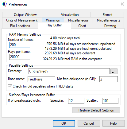
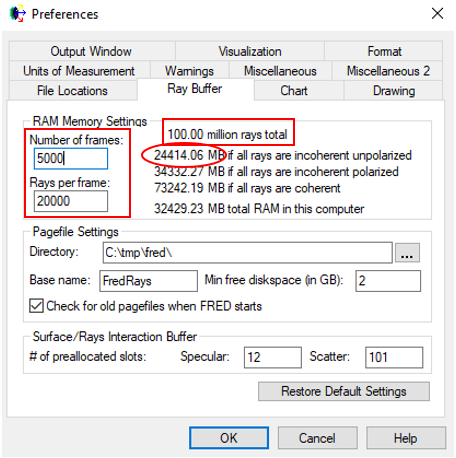
Given the above statements regarding the allocation of RAM to FRED, let us look at a particular case. The Ray Buffer tab of the Preferences dialog is shown below with its default settings. This copy of FRED is installed on a computer having a total of 32GB RAM. The C: drive is an SSD. As shown in the dialog above, FRED will store 20,000 rays in each frame and use 200 frames for a total of 200*20,000 = 4,000,000 rays being stored in RAM at any given moment. If more than 4M rays are generated during a raytrace, the excess rays will be temporarily stored in pagefiles in the C:\tmp\fred\ directory. Furthermore, the 4M rays would consume ~976MB of RAM if they are all incoherent and ~2.9GB of RAM if the rays are all coherent.Let us now modify the ray buffer preferences to take advantage of the 32GB of RAM available on this computer. We don’t want FRED to use all 32GB of RAM, since Windows needs a certain amount of RAM to operate by itself (say 2-3GB) and we may want the computer running other applications in addition. So, let us say that we want FRED to use ~25GB of RAM for storing ray data (and assume these are incoherent rays). In the image below, I have adjusted the number of frames to be 5000, such that I can store 100 million rays in RAM at any given time. I can expect that the 100 million rays will consume 24.4 GB of RAM and that any additional rays will be stored in pagefiles in the C:\tmp\fred\ directory. While the pagefile location has no impact on performance in this case, since the C: drive is an SSD, it does allow put the pagefiles in a directory that is easier for me to find and keep an eye on. Another option worth considering in this dialog is the “Min free disk space (in GB)” setting. By default, FRED requires at least 2GB of free disk space in the pagefile directory to initiate a ray trace. In practice, this error is rarely encountered, but adjusting this value may be beneficial in specific scenarios.
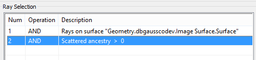
Each Analysis Surface and Detector Entity includes an option to filter the rays contributing to the calculated quantity. This option is located at the bottom of the next image under the section labeled "Ray Selection."
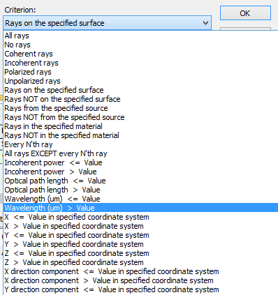
There are many options to choose from:
A very simple way to isolate the stray light contribution in an imaging system (where no scatter is present) is to append a Ray Filter "Specular Ancestry > 0." Thus the designed optical path will be ignored when processing the calculated quantity (e.g. Irradiance). You can append filters by right-clicking in the list area.
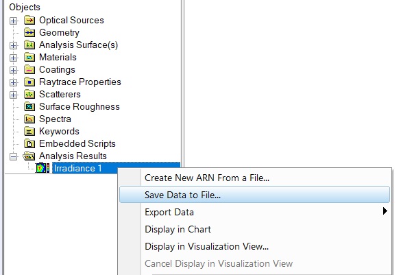
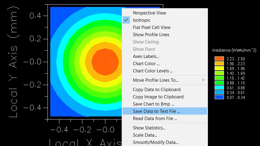
The two pictures below show an Irradiance plot of an imaging system first with and then without the Specular ancestry > 0 filter.
Alternatively, if you wanted to isolate only the scatter contribution you might want to add the Ray Filter "Scatter Ancestry > 0."
This guide explains the concept of ray ancestry in the context of both specular and scattering events, providing graphical illustrations to clarify the associated conventions.
Ray ancestry refers to the splitting of an incident ray into transmitted, reflected, and/or scattered rays. Terms like parent, child, grandchild, and so on—or numerical generations [0, 1, 2, …]—are commonly used to describe this relationship. Control over ray ancestry settings is managed through the Raytrace Controls options.
When a ray is incident upon an interface between two materials of differing refractive index, it undergoes specular splitting into a reflected and transmitted ray if the angle of incidence is less than the critical angle. The parentage of these rays is determined by the Parent Ray Specifier option on the assigned Raytrace Control dialog. The default setting for this option is the Largest incoherent power which is determined by the Coating specification. If the Coating is of type Uncoated, Thin Film, Quarterwave Layer, or General Sampled then the angle of incidence will also play a part in determining which ray is the parent. The user has three other choices for the Parent Ray Specifier: Transmitted [transmitted ray always parent], Reflected [reflected ray always parent], or Monte-Carlo (1 ray only) [probabilistic determination].
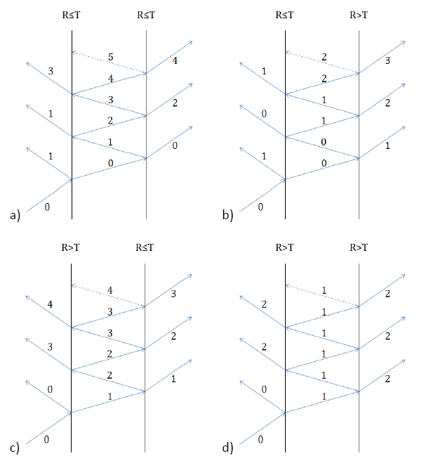
The picture below illustrates graphically the parentage of specular split rays incident on two interfaces under four distinct conditions when Largest incoherent power is selected. When both interfaces have R ≤ T as in Figure a, the parent ray (0) is transmitted along with even generations while the reflected rays are of odd generation. With R ≤ T on the first and R > T on the second as in Figure b, the parent ray is ultimately reflected and increasing generations both reflect and transmit. With R > T on the first and R ≤ T on the second as in Figure c, the parent ray is immediately reflected and increasing generations both reflect and transmit. Finally, with R > T on both interfaces as in Figure d, the parent is immediately reflected with all subsequent reflections and transmissions of generation two.
User Tools enable you to link custom scripts to buttons on FRED's main toolbar. Once configured, you can execute your script with a single click on the associated toolbar button.
To add an existing FRED script to the User Tools toolbar: Go to View > Customize in the menu. In the Customize dialog, select the Toolbars tab. Check the box next to User Tools in the list to enable the toolbar.
Note: To move any toolbar in FRED from its default location, hover your mouse over the vertical ellipse to the left of the toolbar. Hold down the mouse button, drag the toolbar to your preferred location, and release the button when it's positioned as desired.
4. Finally, provide text for the tooltip that displays when you hover your mouse over the button. Use the scroll bar to find and select the corresponding Displayed Name. User Tool #. Type your text in the File Location text box. Click on the OK button to save your changes and close the dialog box.
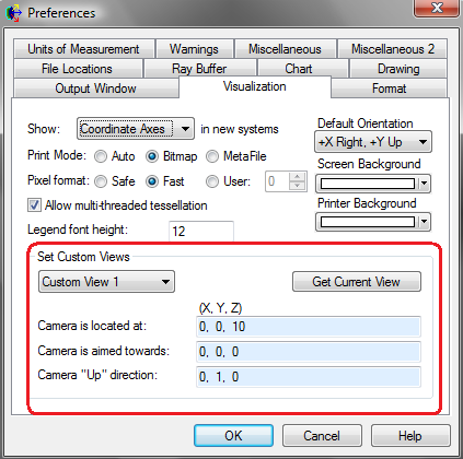
The Visualize toolbar has a dropdown list and several buttons that can be used to quickly snap the 3D View to a specific orientation relative to the global axes. Clicking on one of those buttons, or selecting one of the many options in the dropdown list immediately changes the orientation of the 3D view (e.g., side view, from top, from back, etc.).
The three custom views at the bottom of the dropdown option list allow the user to customize a specific view that can be snapped to this orientation with a single click.
The user can also set the three "Custom View" options in FRED's Preferences by selecting Tools > Preferences from the menu. On the Visualization tab, the user can 1) enter the camera position/orientation manually, or 2) click on the Get Current View button to import the data for the current view.
Analysis Surface Ray Filters provide a method for sorting through rays and establishing a set of criteria that must be met for a ray to be included in the operation being performed (e.g. Irradiance calculation, Spot Diagram).
The video and example file below describes the basic principle behind Ray Selection Filter Criteria.
Ray filters can be specified in the ray selection list by right-mouse clicking and choosing an appropriate option; cut, copy, paste, delete, edit, insert, or append. The specific ray filters are logical operations that evaluate to either TRUE or FALSE on a given ray. Additionally, there is no parenthetical grouping of the ray filters, so they are evaluated sequentially in the list.
Consider the following examples in which a ray selection criteria list consisting of three filters is applied to a single ray. The ray selection criteria list is shown on the left and its logical application to the single ray is shown on the right. In the top example the serial evaluation of AND-AND-OR results in TRUE, meaning that the ray passes the selection criteria and is included in the analysis or operation. In the bottom example the serial evaluation of AND-AND-AND results in a FALSE, meaning that the ray does not pass the selection criteria and is not included in the analysis or operation.
Sometimes rays unexpectedly halt on a surface. The picture below shows a single ray bouncing inside a perfectly reflecting cylinder, but surprisingly stops.
Raytrace Summary
In simple scenarios, looking at the Raytrace Summary that is automatically printed to the Output Window might give you all the information you need. The clue to this problem is in the line "Num rays halted due to exceeding number of consecutive intersections on the same surface."
Table of Ray Errors
In more complex cases, it might be more insightful to view the Table of Ray Errors report located under the Tools menu. This logs all ray errors on a surface-by-surface basis.
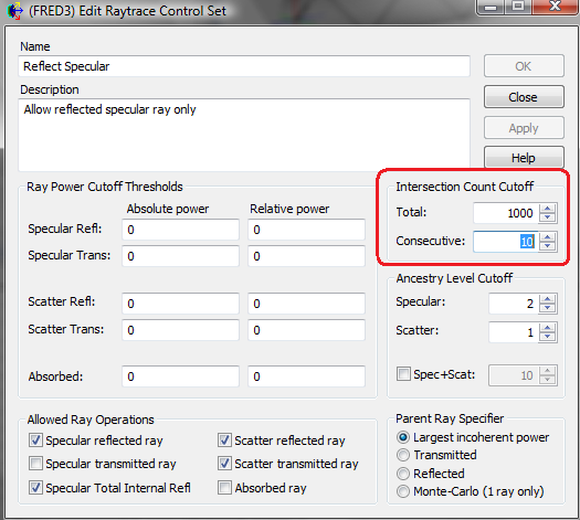
The Solution (in this case)
In this case, we need to increase the relevant cut-off in the associated Raytrace Control, to allow the ray to reflect off the same surface consecutively more than the default 10 times.
FRED supports the import of the following file formats:
STEP (.step, .stp)
IGES (.iges, .igs)
OBJ (.obj)
STL (.stl)
These formats enable seamless integration of CAD-generated geometry into FRED for optical analysis and simulation. If you require additional file format support or encounter any issues during import, please contact our team for assistance.
FRED has no fundamental limits on the number of rays that can be traced or the size of the model, enabling it to handle large-scale simulations efficiently.
For enhanced performance:
FRED Optimum and FRED MPC offer a Distributed Computing option, allowing you to share the raytrace workload across multiple computers.
GPU Raytracing: If multiple GPU boards are available, FRED can utilize them in parallel to further accelerate the raytracing process.
This flexibility ensures efficient processing for complex and demanding optical simulations.
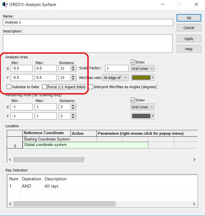
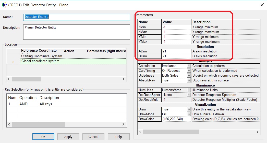
The pixel size of your Analysis Surface and Detector Entities are set in the areas highlighted in the screenshots below.
The pixel size will be the full width of the detector divided by the number of divisions, which in the first case below would be 1/21 = 0.0476mm. If you are using the Analysis Surface, then make sure to uncheck the "Autosize to Data" option to get explicit control over the grid widths, otherwise, FRED will auto size the grid based on the footprint of the ray bundle.
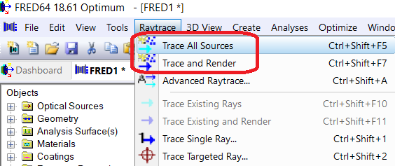
The two primary options for starting a CPU-based raytrace in FRED are "Trace and Render" and "Trace All Sources."
"Trace and Render" displays the rays as they are traced through the system, providing a visual representation of the ray paths.
"Trace All Sources" performs the trace without visualizing the rays, which can improve performance.
While visualizing the rays can be useful, it is important to note that drawing the rays can slow down the raytrace, especially when dealing with large numbers of rays (thousands or millions). For this reason, most users opt for the "Trace All Sources" option when tracing large datasets, as it does not include the overhead of ray visualization.
However, the impact of selecting "Trace and Render" over "Trace All Sources" can be more significant than just a slight slowdown. Enabling ray visualization in "Trace and Render" forces the raytrace to be single-threaded. In contrast, when using "Trace All Sources", FRED can distribute the raytrace across up to 17 threads (cores). For FRED Optimum and FREDmpc, this capability extends even further, utilizing up to 63 threads.
Thus, when multiple cores are available, the difference in performance between "Trace and Render" (single-threaded) and "Trace All Sources" (multi-threaded) can be substantial. The choice of which option to use depends on whether you prioritize visualization or performance.
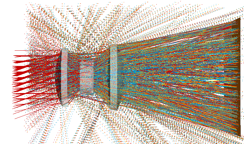
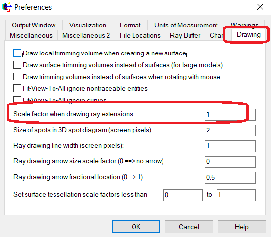
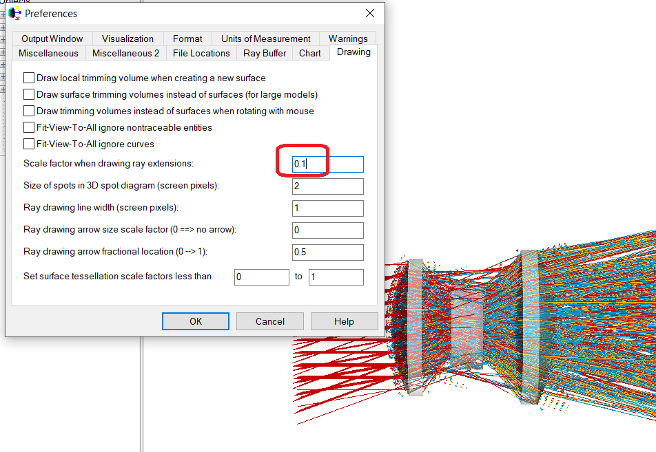
When the user uses the Trace and Render option, rays with dashed lines can sometimes be seen. These are rays that are leaving a surface (or source) and do not intersect with any other surface in the model (i.e. are heading to infinity).
The length of these lines can be decreased (or increased) in the software preferences. To turn off drawing these rays, set this value to 0.
Below is a picture of the same raytrace, with the above scale factor set to 0.1.
The Stray Light Report and the Raytrace Paths Report, both available by selecting Tools > Reports from the FRED menu, are very useful tools for looking at ghost/scatter paths in the system.
If these options are grayed out, it is because you must first perform a raytrace using the Advanced Raytrace dialog with the "Determine raypaths" option selected.
The reports rely on raypath information, which is not automatically saved during a "normal" raytrace. This option must be selected in the Advanced Raytrace settings, as shown below:
Note: It is also valuable to select the "Create/use ray history file" option as discussed in this article: Raypaths and ray history
A non-network license of FRED can be operated via Remote Desktop, as long as the dongle is located on the PC that will be running FRED. The default installation of the software and key driver is required on the host machine.
Additionally, for older superpro dongles, before the dongle will allow you to start a new instance of FRED on the remote machine you will need to make some modifications to how the host computer searches for the dongle. Please take the following actions:
Install the Safe-Net Sentinel services on the machine being used to run FRED. In the FRED installation directory, you will see a Utilities folder which contains the Sentinel Protection Installer. Unplug your hardware dongle and run this installer.
If the computer does not have the Sentinel key software installed, then accept the license agreement and proceed with a CUSTOM install when prompted. In the custom setup step, select each component (Sentinel System Drivers, Sentinel Protection Server, Sentinel Keys Server, and Sentinel Security Runtime) and choose, “This feature, and all subfeatures, will be installed on the local hard drive”. There should be no components with an X symbol present. Hit Next and complete the installation. This process may require you to reboot your computer.
If the computer already has the Sentinel key software installed, select the MODIFY option after running the installer. In the custom setup step, select each component (Sentinel System Drivers, Sentinel Protection Server, Sentinel Keys Server, and Sentinel Security Runtime) and choose, “This feature, and all subfeatures, will be installed on the local hard drive”. There should be no components with an X symbol present. Hit Next and complete the installation. This process may require you to reboot your computer.
After restarting the computer, set up a new system environment variable having name = NSP_HOST and value = RNBO_SPN_LOCAL. Environment variables are accessed through the System dialog found on the Control Panel.
Start FRED locally on the machine to verify that the key is properly detected and that you can run FRED without going over the network.
If (3) is successful, close FRED and log out of the machine.
On another computer, remote the desktop into the machine you just set up and try to start FRED.
This opens the Sentinel Admin Control Center. Choose the "Sessions" option to see the machines currently connected to licenses. To review how many licenses are in use (logins) and available (concurrency) see the information in the "Features" area.
This opens up the Sentinel License Monitor (will install Java if not already on there) which will allow the viewer to see the available licenses and who is using them. Clicking on the leftmost column (Keys#) will show a separate page indicating who is accessing that license. Clicking on the “Sublicense” column will show a separate page indicating how many of the network licenses for that key are in use.
When debugging a script, it's sometimes valuable to check the value of a variable or the contents of a structure or array. This can be done quite easily in FRED's scripting editor.
However, the one thing to note is that you have to specify each item "to watch" individually - you can't just browse the whole of an array or structure
Open the script editor
Left-click in the gray margin at the left side to add a breakpoint at a line of your choosing
Run the script
In the area at the top, note that there is a tab on the left side labeled "Watch", click this.
Then, in the blank window, write in the variables that you wish to keep an eye on. In the picture at the top of this page, there are three examples:
a single variable: lens
a member of the T_ENTITY structure: ent.name
the contents of one cell of an array: myArray(2)
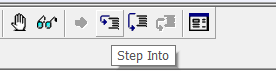
Then as you step through the script (e.g. by using the "step into" button) the value of these variables will be dynamically updated at the top.
Note: if you don't see this mini toolbar at the top of the script debug window, then select from the FRED main menu select Tools / Preferences... / Format tab/ Script Editor Window / Show toolbar
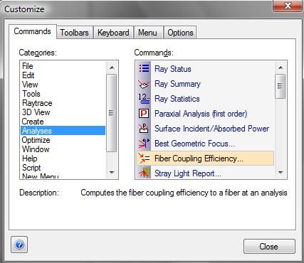
FRED's main toolbar can be customized to suit your needs.
1. Go to View / Customize.. 2. Select Toolbars
Here you can choose which toolbar groupings you want to include on the FRED toolbar.
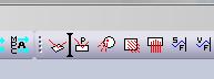
To customize the content of each toolbar grouping: 3. Click back to the Commands tab 4. Select the Category that you wish to customize (e.g. Analyses) 5. To add a button, drag and drop the item from this list to the FRED toolbar
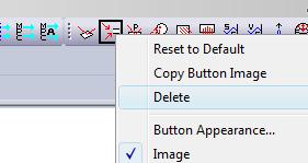
6. To remove a button from the toolbar right-click on the toolbar button and select Delete
Notice also that you can move the toolbars around by dragging them with the mouse.
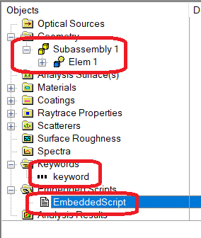
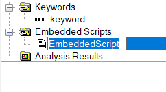
Many items on the Object Tree have setting windows that pop up when you double-click. However some items do not (e.g. a Subassembly, Custom Element, Keyword, Embedded Script, ARN), and therefore it can be a little confusing how to change the name of these items.
You can either highlight the item and the left-click again to edit the name, or highlight the item and press F2 on the keyboard.
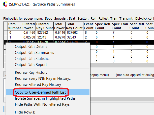
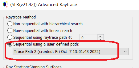
FRED's default raytrace mode is non-sequential, but the user also has the option to switch to a sequential raytrace. One common scenario is that a user might have performed a non-sequential raytrace and is viewing the Raytrace Paths Report, or Stray Light Report and having identified a path of interest will next want to trace it sequentially.
First, right-click on the path of interest and select Copy to User-Defined Path List.
Next, open the Advanced Raytrace dialog (again), and switch the Raytrace Method to "Sequential using a user-defined path", choosing the path that has just been saved.
Note: the path details can be viewed/edited via Raytrace / User-defined Ray Paths...